Alpha Compositing
Transparency may not seem particularly exciting. The GIF image format which allowed some pixels to show through the background was published over 30 years ago. Almost every graphic design application released in the last two decades has supported the creation of semi-transparent content. The novelty of these concepts is long gone.
With this article I’m hoping to show you that transparency in digital imaging is actually much more interesting than it seems – there is a lot of invisible depth and beauty in something that we often take for granted.
Opacity
If you ever had a chance to look through rose-tinted glasses you may have experienced something akin to the simulation below. Try dragging the glasses around to see how they affect what’s seen through them:
The way these kind of glasses work is that they let through a lot of red light, a decent amount of blue light, and only some amount of green light. We can write down the math behind these specific glasses using the following set of three equations. The letter R is the result of the operation and the letter D describes the destination we’re looking at. The RGB subscripts denote the red, green, and blue color components:
RG = DG × 0.7
RB = DB × 0.9
This stained glass lets through red, green, and blue components of the background with different intensities. In other words, the transparency of the rose-tinted glasses depends on the color of the incoming light. In general, transparency can vary with a wavelength of light, but in this simplified situation we’re only interested in how the glasses affect the classic RGB components.
A simulation of the behavior of regular sunglasses is much less complicated, they usually just attenuate some amount of the incoming light:
These sunglasses let through only 30% of the light passing through them. We can describe this behavior using these equations:
RG = DG × 0.3
RB = DB × 0.3
All three color components are scaled by the same value – the absorption of the incoming light is uniform. We could say that the dark glasses are 30% transparent, or we could say that they’re 70% opaque. Opacity of an object defines how much light is blocked by it. In computer graphics we usually deal with a simplified model in which only a single value is needed to describe that property. Opacity can be spatially variant like in a case of a column of smoke which becomes more transparent the higher it goes.
In the real world objects with 100% opacity are just opaque and they don’t let through any light. The world of digital imaging is slightly different. It has some, quite literally, edge cases where even solid opaque things can let through some amount of light.
Coverage
Vector graphics deal with pristine and infinitely precise descriptions of shapes that are defined using points, linear segments, Bézier curves, and other mathematical primitives. When it comes to putting the shapes onto a computer screen, those immaculate beings have to be rasterized into a bitmap:

Rasterization of a vector shape into a bitmap
The most primitive way to do it is to check if a pixel sample is on the inside or on the outside of the vector shape. In the examples below you can drag the triangle on either zoomed or un-zoomed side, the latter lets you perform finer movements. The blue outline symbolizes the original vector geometry. As you can see the steps on the edges of the triangle look unpleasant and they flicker heavily when the geometry is moved:
The flaw of this approach lies in the fact that we only do one test per output pixel and the results are quantized to one of the two possible values – in or out.
We could sample the vector geometry more than once per pixel to achieve a higher gradation of steps and decide that some pixels are covered only partially. One approach is to use four sample points which lets us represent five different levels of coverage: 0, 1/4, 2/4, 3/4, and 1:
The quality of the edges of the triangle is improved, but just five possible levels of coverage are very often not enough and we can easily do a much better job. While describing a pixel as a little square is frowned upon in a world of signal processing, in some contexts it is a useful model that lets us calculate an accurate coverage of a pixel by the vector geometry. An intersection of a line with a square can always be decomposed into a trapezoid and a rectangle:

A linear segment splits a square into a trapezoid and a rectangle
The area of those two parts can be calculated relatively easily and their sum divided by the square’s area specifies the percentage of a coverage of a pixel. That coverage is calculated as an exact number and can be arbitrarily precise. The demonstration below uses that method to render significantly better looking edges that stay smooth when the triangle is dragged around:
When it comes to more complicated shapes like ellipses or Bézier curves, they’re very often subdivided to simple linear segments allowing the coverage evaluation with as high accuracy as required.
Partial coverage is crucial for high quality rendering of vector graphics, including, most importantly, the rendering of text. If you look up close on a screenshot of this page you’ll notice that almost all the edges of the glyphs end up covering the pixels only partially:

Text rendering heavily relies on partial coverage
With the object’s opacity in one hand and its coverage of individual pixels in another, we’re ready to combine them into a single value.
Alpha
The product of an object’s opacity and its pixel coverage is known as alpha:
An object that’s 60% opaque that covers 30% of a pixel’s area has an alpha value of 18% in that pixel. Naturally, when an object is transparent, or it doesn’t cover a pixel at all, its value of alpha at that pixel is equal to 0. Once multiplied the distinction between the opacity and the coverage is lost which in some sense justifies the synonymous use of the terms “alpha” and “opacity”.
Alpha is often presented as a fourth channel of a bitmap. The usual values of red, green, and blue are accompanied by the alpha value to form the quadruple of RGBA values.
When it comes to storing the alpha value in memory one could be tempted to use only a few bits. If you consider the pixel coverage of edges of opaque objects 4 or even 3 bits of alpha often look good enough, depending on the pixel density of your display:
However, opacity also contributes to the alpha value so a low bit-depth may be catastrophic for quality of some smoothly varying transparencies. In the visualization below a gradient spanned between an opaque black and a clear color shows that low bit-depths result in very banded images:
Clearly, the more bits the better and most commonly an alpha bit-depth of 8 is used to match the precision of the color components making many RGBA buffers occupy 32 bits per pixel. It’s worth pointing out that unlike the color components which are often encoded using a non-linear transformation, alpha is stored linearly – encoded value of 0.5 corresponds to alpha value of 0.5.
So far when talking about alpha we’ve completely ignored any color components, but other than blocking a background color a pixel can add some color on its own. The idea is fairly simple – a semi-transparent pink object blocks some of the incoming background light and emits, or reflects, some of the pink light:
Note that this behaves differently from a stained glass. The glass merely blocks some of the background light with varying intensities. Looking at a pitch black object with rose-stained glass maintains the blackness since a black object doesn’t emit or reflect any light in the first place. However, the semi-transparent pink object adds its own light. Placing it on top of a black object produces a pinkish result. A good equivalent of that behavior is a fine material suspended in the air, be it haze, smoke, fog, or some colorful powder.
Visualizing the alpha channel is a little complicated – a perfectly transparent object is by definition invisible, so I’ll use two tricks to make things discernible. A checkerboard background shows which parts of the image are clear, a pattern used in many graphic design applications:

Checkerboard pattern showing clear parts
The four little squares under the image tell us we’re looking at red, green, blue, and alpha components of the image. In some cases it’s useful to see the values of the alpha channel directly and the easiest way to present them is by using shades of gray:

Showing RGB and A values as separate planes
The brighter the gray the higher the alpha value and so pure black corresponds to 0% alpha and pure white means 100% alpha. The little squares show that RGB and A components of the image have been separated into two planes.
On its own the alpha component isn’t particularly useful, but it becomes critical when we talk about compositing.
Simple Compositing
Very few 2D rendering effects can be achieved with a single operation and we use the process of compositing to combine multiple images to create the final output. As an example, a simple “Cancel” button can be created by a composition of five separate elements:

Compositing elements of a “Cancel” Button
Compositing is often performed in multiple steps where each step combines two images. The usual name for the foreground image being composed is a source. The background image that is being composed into is called a destination. It’s easy to remember if you think of it in terms of the new pixels from the source arriving at the destination.
We’ll start with compositing against an opaque background since it is a very common case. Everything you see on your screen ultimately ends being composited into a non-transparent destination.
When the value of alpha of the source is 100% the source is opaque and it should cover the destination completely. For the alpha value of 0% the source is completely transparent and the destination should not be affected. Alpha value of 25% allows the object to emit 25% of its light and lets through 75% of the light from the background and so on:

Compositing of purple sources with various alpha values into a yellow destination
You may see where this is all going – the simple case of alpha compositing against an opaque background is just a linear interpolation between the destination and the source colors. In the chart below the slider controls the alpha value of the source, while the red, green, and blue plots depict the values of the RGB components. The result R is just a mix between the source S and the destination D:
We can describe what’s going on using the following equations. As before, the subscript denotes the component, so SA is the alpha value of the source, while DG is the green value of the destination:
RG = SG × SA + DG × (1 − SA)
RB = SB × SA + DB × (1 − SA)
The equations for the red, green, and blue components have the same form so we can just use an RGB subscript and combine everything into a single line:
Moreover, since the destination is opaque and already blocks all the background light we know that the alpha value of the result is always equal to 1:
Compositing against an opaque background is simple, but unfortunately quite limited. There are many cases where a more robust solution is needed.
Intermediate Buffers
In the image below you’ll see a two step process of compositing three different layers marked as: A, B, and C. I’ll use symbol ⇨ to denote “composed onto”:

Compositing result of three layers in two steps
We first compose B onto C, and then we compose A onto that to achieve the final image. In the next example we’re going to do things slightly differently. We’ll compose the two topmost layers first, and then we’ll compose that result into the final destination:

Compositing result of three layers in two steps with different order
You may wonder if that situation happens in practice, but it’s actually very common. A lot of non-trivial compositing and rendering effects like masking and blurring require a step through an intermediate buffer that contains only partial results of compositing. That concept is known under different names: offscreen passes, transparency layers, or side buffers, but the idea is usually the same.
More importantly, almost any image with transparency can be thought of as a partial result of some rendering that, at some later time, will be composed to its final destination:
Partial composition of a button into a buffer
We want to figure out how to replace the composition of semi-transparent images A and B with a single image (A⇨B) that will have the same color and opacity. Let’s start by calculating the alpha value of the resulting buffer.
Combining Alphas
It may be unclear how to combine opacities of two objects, but it’s easier to reason about the issue when we think about the transparencies instead.
Consider some amount of light passing through a first object and then through a second object. If the transparency of the first object is 80%, it will let through 80% of the incoming light. Similarly, a second object with transparency 60% will let through 60% of the light passing through it, which is 60% × 80% = 48% of the original light. You can try this in a demonstration below, remember that the sliders control transparency and not opacity of the objects in the path of light:
Naturally, when either the first or the second object is opaque no light passes through even when the other one is fully transparent.
If an object D has transparency DT and object S has transparency ST, then the resulting transparency RT of those two objects combined is equal to their product:
However, transparency is just one minus alpha, so a substitution gets us:
Which expands to:
And simplifies to:
This can be further minimized to one of the two equivalent forms:
RA = DA + SA × (1 − DA)
We’ll soon see that the former is more commonly used. As an interesting side note, notice that the resulting alpha doesn’t depend on the relative order of the objects – the opacity of the resulting pixels is the same even when the source and destination are switched. This makes a lot of sense. A light passing through two objects should be equally dimmed when it’s shining front to back or back to front.
Combining Colors
Calculating alpha wasn’t that difficult so let’s try to reason through the math behind the RGB components. The source image has a color SRGB, but its opacity SA causes it to contribute only the product of those two values to the final result:
The destination image has a color DRGB, its opacity causes it to emit DRGB×DA light, however, some part of that light is blocked by opacity of S so the entire contribution from the destination is equal to:
The total light contribution from both S and D is equal to their sum:
Similarly, the contribution of the merged layers is equal to their color times their opacity:
We want those two values to match:
Which gives us the final equations:
RRGB = (SRGB×SA + DRGB×DA×(1 − SA)) / RA
Look how complicated the second equation is! Notice that to obtain the RGB values of the result we have to do a division by the alpha value. However, any subsequent compositing step will require a multiplication by the alpha value again, since the result of a current operation will become a new source or destination in the next operation. This is just inelegant.
Let’s go back to the almost final form of RRGB for a second:
The source, the destination, and the result are multiplied by their alpha components. This hints us that the pixel’s color and its alpha like to be together, so let’s try to take a step back and rethink the way we store the color information.
Premultiplied Alpha
Recall how we talked about opacity – if the object is partially opaque the contribution of its color to the output is also partial. Premultiplied alpha makes this idea explicit. The values of the RGB components are, as the name implies, premultiplied by the alpha component. Starting with a non-premultiplied color:
Alpha premultiplication results in:
Let’s look at more than one pixel at the time. The following picture shows how color information is stored in a non-premultiplied alpha:

RGB and A information in a non-premultiplied image
Notice that the areas where alpha is 0 can have arbitrary RGB values as shown by the green and cyan glitches in the image. With premultiplied alpha the color information also carries the values of pixel’s opacity:

RGB and A information in a premultiplied image
Premultiplied alpha is sometimes called associated alpha, while non-premultiplied alpha is occasionally referred to as straight or unassociated alpha.
When the alpha component of a color is equal to 0, the premultiplication nullifies all the other components, regardless of what was in them:
With premultiplied alpha there is only one completely transparent color – a charming simplicity.
The benefits of this treatment of color components may slowly start to become clear, but before we go back to our compositing example let’s see how premultiplied alpha helps to solve some other rendering issues.
Filtering
A gaussian blur is a popular way to either provide an interesting unfocused background, or as a way of reducing the high frequency of the underlying contents in some UI elements. As we’ll see alpha premultiplication is critical to achieve correctly looking blurs.
The image we’ll analyze is created by filling the background with 1% opaque blue color and then painting an opaque red circle on top. First, let’s consider a non-premultiplied example. I separated RGB channels from the alpha channel to make it easier to see what’s going on. The arrow symbolizes the blur operation:
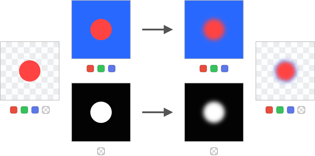
Blurring non-premultiplied content
The final result has an ugly blue halo around it. This happens because the blue background seeps into the red area during the blur and then it’s weighted by the alpha at composite time.
When the colors are alpha premultiplied the final result is correct:
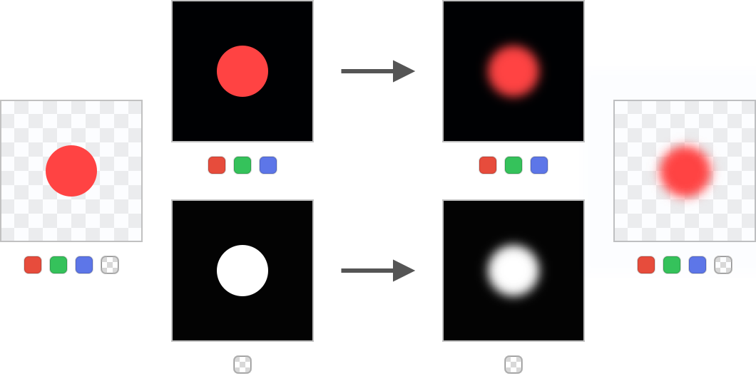
Blurring premultiplied content
Due to the premultiplication the blue color in the image is reduced to 1% of its original strength so its impact on the colors of the blurred circle is expectedly minimal.
Interpolation
Rendering an image whose pixels are perfectly aligned with a destination is easy since we have a trivial one-to-one mapping between the samples. A problem arises when the simple mapping doesn’t exist, e.g. due to rotation, scaling, or translation. In the picture below you can see how the pixels of a rotated image shown with a red outline no longer align with a destination:

Relative orientation of image and destination pixels before and after rotation
There are multiple ways of deciding which color from the image should be put into the destination pixel and the easiest option is a so called nearest-neighbor interpolation which simply chooses the nearest sample in the texture as the resulting color.
In the demonstration below the red outline shows the position of the image in the destination. The right side presents the sample positions from the point of view of the image. By dragging the slider you can rotate the quad to see how the samples pick up colors from the bitmap. I highlighted a single pixel in both the source and the destination to make it easier to see how they relate:
That approach works and the pixels are consistently colored, but the quality is unacceptable. A better way to do it is to use bilinear interpolation which calculates a weighted average of the four nearest pixels in the sampled image:
This is better, but the edges around the rectangles just don’t look right, the contents of the non-premultiplied pixels bleeds in since the alpha is “applied” after interpolation. The sometimes recommended approach of bleeding the color of the valid contents out, which you can see some examples of in Adrian Courrèges' fantastic article, is far from perfect – no color would make the one pixel gap between the red and the blue rectangle look correct.
Let’s see how things look when an image is alpha premultiplied, and, to foreshadow a little, composited using a better equation that we’ll derive in a minute:
It’s just perfect, we got rid of all the color bleeding and jaggies are nowhere to be seen.
The issues related to blurring and interpolation are ultimately closely related. Any operation that requires some combination of semi-transparent colors will likely have incorrect results unless the colors are alpha premultiplied.
Compositing Done Right
Let’s jump back to compositing. We’ve left the discussion with the almost finished derivation:
If we represent the colors using premultiplied alpha all those pesky multiplications disappear since they’re already part of the color values and we end up with:
Let’s have a look at the equation for the alpha:
The factors for red, green, blue, and alpha channels are all the same, so we can just express the entire thing using a single equation and just remember that every component undergoes the same operation:
Look how premultiplied alpha made things beautifully simple. When we analyze the components of the equation they all fit right in. The operation masks some background light and adds new light:
This blending operation is known as source-over, sover, or just normal, and, without a doubt, it is the most commonly used compositing mode. Almost everything you see on this website was blended using this mode.
Associativity
An important feature of the source-over on premultiplied colors is that it’s associative. In a complex blending equation this lets us put the parentheses completely arbitrarily. All compositions below are equivalent:
R = (A⇨B)⇨(C⇨(D⇨E))
R = A⇨(B⇨(C⇨(D⇨E)))
The proof is fairly simple, but I won’t bore you with the algebraic manipulations. The practical implication is that we can perform partial renders of complicated drawings without a fear that the final composition will look any different.
The vast majority of time the alpha is used purely for source-over compositing, however, its power doesn’t stop there. We can use the alpha values for other useful rendering operations.
Porter-Duff
In July 1984 Thomas Porter and Tom Duff have published a seminal paper entitled “Compositing Digital Images”. The authors not only introduced the concept of premultiplied alpha and derived the equation behind source-over compositing, but they also presented an entire family of alpha compositing operations, many of which are not well know despite being very useful. The introduced functions are also known as operators, since, similarly to addition or multiplication, they operate on input values to create an output value.
Over
In the following examples we’ll use the interactive demos that show how different blend modes operate. The destination has a black clubs symbol ♣, while the source has a red hearts symbol ♥. You can drag the heart around to see how the overlap of the two shapes behaves under different compositing operators. Notice the little minimap in the corner. Some blend modes are quite destructive and it may be easy to lose track of what’s where. The minimap always shows a result of the simple source-over compositing which should make it easier to navigate:
If you switch to destination-over you’ll quickly realize it’s just a “flipped” source-over, the destination and source swap places in the equation and the result is equivalent to treating the source as the destination and the destination as the source. While seemingly redundant, the destination-over operator is quite useful as it lets us composite things behind already existing contents.
Out
The source-out and destination-out operators are great for punching holes in the source and destination respectively:
Destination-out is the more convenient operator of the two, it uses the alpha channel of the source to punch out the existing destination.
In
The source-in and destination-in are essentially masking operators:
They make it fairly easy to obtain complex intersections of complicated geometry without resolving to relatively difficult to compute intersections of vector-based paths.
Atop
The source-atop and destination-atop allow overlaying of new contents on top of existing one, while simultaneously masking it to the destination:
Xor
The exclusive-or operator or just xor keeps either the source or the destination, their overlap disappears:
Source, Destination, Clear
The last three classic compositing mode are rather dull. Source, also known as copy just takes the source color. Similarly, destination ignores the source color and simply returns the destination. Finally, clear simply wipes everything:
The usefulness of those modes is limited. A dirty buffer may be reset using clear which can be optimized to just filling memory with zeros. Additionally, in some cases source may be cheaper to evaluate since it doesn’t require any blending at all, it just replaces the contents of a buffer with source.
Porter-Duff in Action
With the individual operators out of the way let’s see how we can combine them. In the example below we’ll paint a nautical motif in nine steps without using any masking or complex geometrical shapes. The blue outlines show the simple geometry that is emitted. You can advance the steps by clickingtapping on the right half of the image and go back by clickingtapping on the left half of the image:
You should by no means forget about masks and clip paths, but Porter-Duff compositing modes are an often forgotten tool that makes some visuals effects much easier to achieve.
Operators
If you ponder on the Porter-Duff operators we’ve discussed you may notice that they all have the same form. A source is always multiplied by some factor FS and added to the destination multiplied by a factor FD:
Possible values of the FS are 0, 1, DA, and 1 − DA, while FD can be either 0, 1, SA, or 1 − SA. It doesn’t make much sense to multiply the source or destination by their respective alphas since they’re already premultiplied and we’d just achieve a wacky, but not particularly useful alpha-squaring effect. We can present all the operators in a table:
| 0 | 1 | DA | 1 − DA | |
| 0 | clear | source | source-in | source-out |
| 1 | destination | destination-over | ||
| SA | destination-in | destination-atop | ||
| 1 − SA | destination-out | source-over | source-atop | xor |
| 0 | 1 | DA | 1 − DA | |
| 0 | clear | source | source-in | source-out |
| 1 | dest | dest-over | ||
| SA | dest-in | dest-atop | ||
| 1 − SA | dest-out | source-over | source-atop | xor |
| 0 | 1 | DA | 1 − DA | |
| 0 | clear | s | sin | sout |
| 1 | d | dover | ||
| SA | din | datop | ||
| 1 − SA | dout | sover | satop | xor |
Notice the symmetry of the operators along the diagonal. The four central entries in the table are missing and that’s cause they’re unlike the others.
Additive Lighting
In their paper Porter and Duff presented one more operator created when both FS and FD are equal to 1. It’s known as plus, lighter, or plus-lighter:
This operation effectively adds source light to the destination:
Additive light with the plus operator
Green and red correctly created yellow, while green and blue produced cyan. The black color is a no-op – it doesn’t modify the color values in any way since adding zero to a number doesn’t do anything.
The three remaining operators were never named and that’s cause they’re not particularly useful. They’re simply a combination of masking and additive blending.
It’s also worth noting that premultiplied alpha lets us abuse the source-over operator. Let’s look at the equation again:
If we manage to make the alpha value of the source equal to zero, but have non-zero values in RGB channels we can achieve additive lighting without using plus operator:
Additive light with the source-over operator
Note that you have to be careful – the values are no longer correctly premultiplied. Some pieces of software may have an optimization that avoids blending colors with zero alpha completely, while others may un-premultiply the alpha values, do some color operations, and then premultiply again which would wipe the color channels completely. It may also be difficult to export assets in that format, so you should stick to plus unless you control your rendering pipeline completely.
So far all the pieces I’ve talked about have fit together gracefully. Let’s take the rose-tinted glasses off and discuss some of the issues that one should be aware of when dealing with alpha compositing.
Group Opacity
Let’s look at this simple drawing of a pill done using just six primitives:
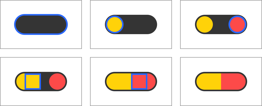
Drawing a pill using simple shapes
If we were asked to render the pill at 50% opacity one could be tempted to just halve the opacity of every drawing operation, however, it proves to be a faulty approach:
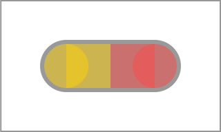
Unexpected rendering of a pill at half opacity
To achieve the correct result we can’t just distribute object’s opacity into each of its individual components. We have to create the object first by rendering it to a bitmap, then modify the opacity of that bitmap, and finally compose:
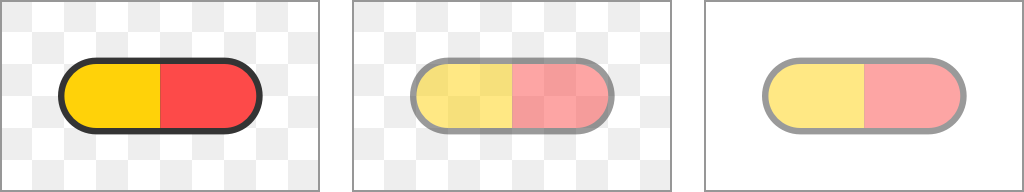
Expected rendering of a pill at half opacity
This is yet another case when the concept of rendering into a side buffer shows its usefulness.
Compositing Coverage
Conversion of geometrical coverage to a single alpha value has some unfortunate consequences. Consider a case in which two perfectly overlapping edges of vector geometry, depicted below with orange and blue outlines, are rendered into a bitmap. In an ideal world the results should look something like this since each pixel is perfectly covered:

An ideal result of rendering with correct coverage
However, if we first render the orange geometry and then the blue geometry the edge pixels of the result will still have some white background bleeding in:

Two-step composited result
Once the coverage is stored in the alpha channel all its geometrical information is lost and there is no way to recreate it. The blue geometry just blends with some contents in the buffer but it simply can’t know that the geometry behind the reddish pixels was intended to match it. This issue is particularly visible when the geometries are perfectly overlapping. In the picture below a white circle is painted on top of black circle. You can see the dark edges despite both circles having the exact same radius and position:

A white circle drawn on top of a black circle
One way to avoid this problem is to not calculate partial coverage of pixels, but instead use significantly scaled-up buffers. By rasterizing the vector geometry with a simple in/out coverage and then scaling the final result down to the original size we can achieve the expected outcome.
However, to perfectly match the quality of edge rendering of an 8-bit alpha channel the buffers would have to be 256 times larger in both directions, an increase in number of pixels by a whooping factor of 216. As we’ve seen, reducing bit-depth for coverage can still produce satisfying results so in practice smaller scales could be used.
It’s worth noting that those issues can often be avoided relatively easily even without using any super-sized bitmaps. For example, instead of drawing two overlapping circles one could just draw two squares on top of each other and then mask the result to the shape of the circle.
Linear Values
If you had a chance to brush up your knowledge of color spaces you may remember that most of them encode the color values nonlinearly and performing correct mathematical operations requires a prior linearization. When that step is done the result of compositing looks as follows, notice they nicely yellowish tint of the overlapping parts:
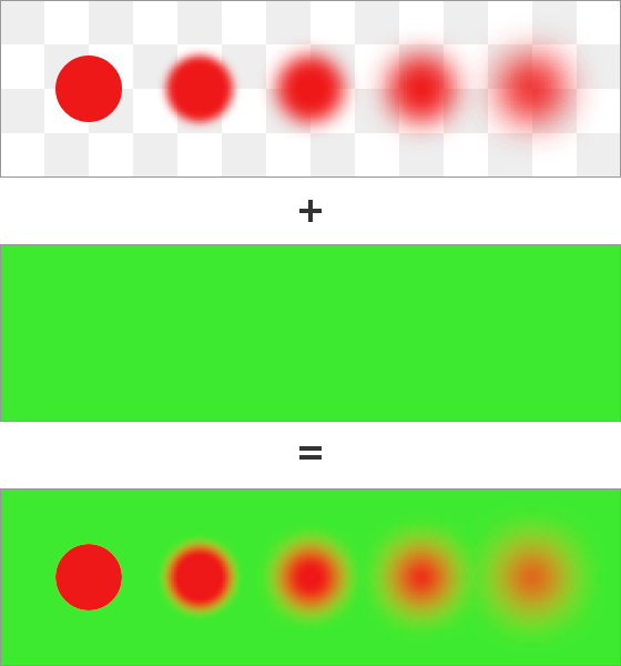
Fuzzy red circles composited on a green background using linear values
For better or for worse, this is not how most compositing works. The default way to do things on the web and in most graphic design software is to directly blend non-linear values:
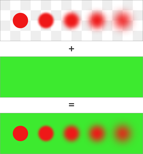
Fuzzy red circles composited on a green background using non-linear values
See how much darker the overlap between the reds and the greens is. This is far from perfect, but there are some cases when doing things incorrectly has become deeply ingrained in the way we think about color. For example, opaque 50% gray from sRGB space looks exactly the same as pure black at 50% opacity blended with a white background:

Composition of two colors against a white background without linearization
In the picture below the sRGB colors from the source and destination are linearized, composited, and then converted back to non-linear encoding for display. This is how those colors should actually look:

Composition of two colors against a white background with linearization
We’ve now introduced a discrepancy that goes against the expectations. The only way to achieve the visual parity using that method is to pick all the colors using linear values, but those are quite different than what everyone is used to. A 50% gray with linear values looks like 73.5% sRGB gray.
Additionally, special care has to be taken when dealing with premultiplied alpha. The premultiplication should happen on the linear values, i.e. before then non-linear encoding happens. This will cause the linearization step to correctly end up with proper alpha premultiplied linear values.
Premultiplied Alpha and Bit Depth
While very useful for compositing, filtering, and interpolation, premultiplied alpha isn’t a silver bullet and has some drawbacks. The biggest one is the reduction of bit-depth of representable colors. Let’s think about an 8-bit encoding of value 150 that is premultiplied by 20% alpha. After alpha premultiplication we get
If we repeat the same procedure for a value of 151 we get:
The encoded value is the same despite the difference in the input value. In fact, values 148, 149, 150, 151, and 152 end up being encoded as 30 after alpha premultiplication, the original distinction between those five unique numbers is lost:

Premultiplication by 20% alpha collapses different 8-bit values into the same one
Naturally, the lower the alpha the more severe the effect is. From the possible range of 2564 (roughly 4.3 billion) different combinations of 8-bit RGBA values only 25.2% of them end up having unique representation after premultiplication, we’re effectively wasting almost 2 bits of the 32 bit range.
Transformation of colors between various color spaces often requires the color components to be un-premultiplied, that is divided by the alpha component, to get the original intensity of the color. That step is mandatory due to already mentioned common non-linear nature of the encoding. The existence of premultiplication reduces the accuracy of color representation and the conversions between color spaces may be imperfect.
In practice the reduction of bit depth is rarely important, especially when it comes to compositing. The lower the alpha value the less visible the color is and the less impactful its compositing becomes. If you’re aiming for pedantically accurate operations on colors you wouldn’t be using 8-bit representation in the first place – the floating point formats are much better suited for this purpose.
Further Reading
The concept of an alpha channel was created by Alvy Ray and Ed Catmull – the cofounders of Pixar. The former’s Alpha and the History of Digital Compositing describes the history of the invention and origins of the name “alpha”, while also showing how those concepts built on and significantly surpassed the matting used in filmmaking.
For a detailed discussion of the meaning of alpha I highly recommend Andrew Glassner’s Interpreting Alpha. His paper provides a rigorous, but very readable mathematical derivation of alpha as an interaction between opacity and coverage.
Finally, for a thorough discourse on premultiplied alpha you can’t go wrong with GPUs prefer premultiplication by Eric Haines. He not only provides a great overview of the issues caused by not premultiplying, especially as they relate to 3D rendering, but also links to a bunch of other articles that discuss the problem.
Final Words
This article originally started as a simple exposé of Porter-Duff compositing operators, but all the other concepts related to alpha compositing were just too interesting to leave by.
One thing I particularly like about the alpha is that it’s just an extra number that accompanies the RGB components, yet it opens up so many unique rendering opportunities. It literally created a new dimension of what could be achieved in the plain old world of compositing and 2D rendering.
The next time you look at smooth edges of vector shapes, or you notice a dark overlay making some parts of a user interface dimmer, remember it’s just a small but mighty powerful component making it all possible.